
26.2. K-Means Clustering: A Larger Example#
Now that we understand the k-means clustering algorithm, let’s try an example with more features and use and elbow plot to choose \(k\). We will also show how you can (and should!) run the algorithm multiple times with different initial centroids because, as we saw in the animations from the previous section, the initialization can have an effect on the final clustering.
Clustering Countries#
For this example, we will use a dataset[1] with information about countries across the world. It includes demographic, economic, environmental, and socio-economic information from 2023. This data and more information about it can be found here. The first few lines are shown below.
countries = pd.read_csv("../../data/world-data-2023.csv")
countries.head()
| Country | Density\n(P/Km2) | Abbreviation | Agricultural Land( %) | Land Area(Km2) | Armed Forces size | Birth Rate | Calling Code | Capital/Major City | Co2-Emissions | ... | Out of pocket health expenditure | Physicians per thousand | Population | Population: Labor force participation (%) | Tax revenue (%) | Total tax rate | Unemployment rate | Urban_population | Latitude | Longitude | |
|---|---|---|---|---|---|---|---|---|---|---|---|---|---|---|---|---|---|---|---|---|---|
| 0 | Afghanistan | 60 | AF | 58.10% | 652,230 | 323,000 | 32.49 | 93.0 | Kabul | 8,672 | ... | 78.40% | 0.28 | 38,041,754 | 48.90% | 9.30% | 71.40% | 11.12% | 9,797,273 | 33.939110 | 67.709953 |
| 1 | Albania | 105 | AL | 43.10% | 28,748 | 9,000 | 11.78 | 355.0 | Tirana | 4,536 | ... | 56.90% | 1.20 | 2,854,191 | 55.70% | 18.60% | 36.60% | 12.33% | 1,747,593 | 41.153332 | 20.168331 |
| 2 | Algeria | 18 | DZ | 17.40% | 2,381,741 | 317,000 | 24.28 | 213.0 | Algiers | 150,006 | ... | 28.10% | 1.72 | 43,053,054 | 41.20% | 37.20% | 66.10% | 11.70% | 31,510,100 | 28.033886 | 1.659626 |
| 3 | Andorra | 164 | AD | 40.00% | 468 | NaN | 7.20 | 376.0 | Andorra la Vella | 469 | ... | 36.40% | 3.33 | 77,142 | NaN | NaN | NaN | NaN | 67,873 | 42.506285 | 1.521801 |
| 4 | Angola | 26 | AO | 47.50% | 1,246,700 | 117,000 | 40.73 | 244.0 | Luanda | 34,693 | ... | 33.40% | 0.21 | 31,825,295 | 77.50% | 9.20% | 49.10% | 6.89% | 21,061,025 | -11.202692 | 17.873887 |
5 rows × 35 columns
We want to see if we can cluster countries based on their characteristics. First, we need to do some cleaning. I don’t want to include Abbreviation, Calling Code, Capital/Major City, Largest city, Latitude, or Longitude in my analysis because they uniquely identify a given country. I also see some variables that are numeric with percentage signs, dollar signs, and commas. These are characters which indicate that the variable is a string, but I would like them to be floats instead so that Python knows they have a numerical meaning.
The code used for this cleaning is hidden for brevity, but the resulting, clean dataframe is shown below.
Show code cell source
countries_clean = countries.drop(columns = ['Abbreviation', 'Calling Code', 'Capital/Major City', 'Largest city', 'Latitude', 'Longitude','Minimum wage'])

def str_to_num(my_input):
    '''Takes in a number in string format and removes commas
    and percentage signs before returning it as a float or int

    If the string is not a number or input is not a string,
    returns the input'''


    if type(my_input) is str:

        cleaned_input = my_input.strip() #strip trailing whitespace
        cleaned_input = cleaned_input.removeprefix("$").removesuffix("%") #remove these characters if they are present

        if cleaned_input.isdigit():
            return int(cleaned_input)
        elif ("." in cleaned_input) and (cleaned_input.replace(".","").replace("-","").isdigit()): #is the only non-digit character a "."
            return float(cleaned_input)
        elif ("," in cleaned_input) and (cleaned_input.replace(",","").replace("-","").isdigit()): #is the only non-digit character a ","
            return int(cleaned_input.replace(",",""))
        elif ("." in cleaned_input) and ("," in cleaned_input) and (cleaned_input.replace(".","").replace(",","").replace("-","").isdigit()): #contains 2 non-digit characters "," and "."
            return float(cleaned_input.replace(",",""))
        else:
            return my_input
    else:
        return my_input

countries_clean = countries_clean.map(str_to_num) #apply this function to every cell in the dataframe
countries_clean = countries_clean.dropna(subset=countries_clean.columns.difference(['Official language','Currency code']),ignore_index = True) #remove rows with any missing numeric values
countries_clean.head()
| Country | Density\n(P/Km2) | Agricultural Land( %) | Land Area(Km2) | Armed Forces size | Birth Rate | Co2-Emissions | CPI | CPI Change (%) | Currency-Code | ... | Maternal mortality ratio | Official language | Out of pocket health expenditure | Physicians per thousand | Population | Population: Labor force participation (%) | Tax revenue (%) | Total tax rate | Unemployment rate | Urban_population | |
|---|---|---|---|---|---|---|---|---|---|---|---|---|---|---|---|---|---|---|---|---|---|
| 0 | Afghanistan | 60 | 58.1 | 652230.0 | 323000.0 | 32.49 | 8672.0 | 149.90 | 2.3 | AFN | ... | 638.0 | Pashto | 78.4 | 0.28 | 38041754.0 | 48.9 | 9.3 | 71.4 | 11.12 | 9797273.0 |
| 1 | Albania | 105 | 43.1 | 28748.0 | 9000.0 | 11.78 | 4536.0 | 119.05 | 1.4 | ALL | ... | 15.0 | Albanian | 56.9 | 1.20 | 2854191.0 | 55.7 | 18.6 | 36.6 | 12.33 | 1747593.0 |
| 2 | Algeria | 18 | 17.4 | 2381741.0 | 317000.0 | 24.28 | 150006.0 | 151.36 | 2.0 | DZD | ... | 112.0 | Arabic | 28.1 | 1.72 | 43053054.0 | 41.2 | 37.2 | 66.1 | 11.70 | 31510100.0 |
| 3 | Angola | 26 | 47.5 | 1246700.0 | 117000.0 | 40.73 | 34693.0 | 261.73 | 17.1 | AOA | ... | 241.0 | Portuguese | 33.4 | 0.21 | 31825295.0 | 77.5 | 9.2 | 49.1 | 6.89 | 21061025.0 |
| 4 | Argentina | 17 | 54.3 | 2780400.0 | 105000.0 | 17.02 | 201348.0 | 232.75 | 53.5 | ARS | ... | 39.0 | Spanish | 17.6 | 3.96 | 44938712.0 | 61.3 | 10.1 | 106.3 | 9.79 | 41339571.0 |
5 rows × 28 columns
Preprocessing the Data#
In the previous section, we wrote our own functions to implement the k-means algorithm. This is a useful exercise to make sure we understand how the algorithm works, but as we know, there are libraries with optimized functions built to do these kinds of common analyses. The library sklearn has built-in functions to do k-means clustering that are much faster than the functions we wrote. Let’s use these functions to cluster our countries dataset.
Before, we can cluster the data, we need to do some preprocessing. Below, I import StandardScaler which we can use to standardize our data.
from sklearn.preprocessing import StandardScaler
Next, we separate our numeric and categorical data for ease of preprocessing.
country_names = countries_clean['Country']
num_columns = countries_clean.drop(columns=['Country', 'Currency-Code', 'Official language'])
cat_columns = countries_clean[['Currency-Code', 'Official language']]
Now, we can use get_dummies from the pandas library to dummy code our categorical features. I set drop_first equal to True so that the first category will be dropped and used as the reference level. I also set dummy_na equal to True which creates a dummy variable to indicate which values are missing.
cat_dummies = pd.get_dummies(cat_columns, drop_first=True, dummy_na=True)
Next, we need to initialize our StandardScaler and use it to scale our numeric features.
scaler = StandardScaler()
num_scaled = pd.DataFrame(scaler.fit_transform(num_columns),columns=num_columns.columns)
Now, we can put our categorical and numerical data back together into one preprocessed dataframe using the .concat function from pandas.
countries_proc = pd.concat([num_scaled,cat_dummies], axis = 1)
countries_proc.head()
| Density\n(P/Km2) | Agricultural Land( %) | Land Area(Km2) | Armed Forces size | Birth Rate | Co2-Emissions | CPI | CPI Change (%) | Fertility Rate | Forested Area (%) | ... | Official language_Swahili | Official language_Swedish | Official language_Tamil | Official language_Thai | Official language_Tok Pisin | Official language_Turkish | Official language_Ukrainian | Official language_Urdu | Official language_Vietnamese | Official language_nan | |
|---|---|---|---|---|---|---|---|---|---|---|---|---|---|---|---|---|---|---|---|---|---|
| 0 | -0.215644 | 0.818138 | -0.115866 | 0.348798 | 1.264388 | -0.232539 | -0.077214 | -0.280488 | 1.414957 | -1.256779 | ... | False | False | False | False | False | False | False | False | False | False |
| 1 | -0.156441 | 0.115295 | -0.389922 | -0.417215 | -0.788460 | -0.236728 | -0.335232 | -0.389776 | -0.774075 | -0.051855 | ... | False | False | False | False | False | False | False | False | False | False |
| 2 | -0.270901 | -1.088910 | 0.644351 | 0.334160 | 0.450584 | -0.089375 | -0.065003 | -0.316917 | 0.301239 | -1.317025 | ... | False | False | False | False | False | False | False | False | False | False |
| 3 | -0.260376 | 0.321462 | 0.145437 | -0.153746 | 2.081166 | -0.206181 | 0.858093 | 1.516694 | 2.221443 | 0.791591 | ... | False | False | False | False | False | False | False | False | False | False |
| 4 | -0.272217 | 0.640084 | 0.819584 | -0.183020 | -0.269053 | -0.037369 | 0.615715 | 5.936791 | -0.282503 | -0.899936 | ... | False | False | False | False | False | False | False | False | False | False |
5 rows × 192 columns
Choosing K#
Now that our data has been preprocessed, we are ready to start clustering. First, we import the KMeans function from sklearn.cluster.
from sklearn.cluster import KMeans
The KMeans function takes in the number of clusters, \(k\), as n_clusters, the number of times the algorithm should be run with different initial centroids as n_init, and a random seed (as explained in Section 10.3) as random_state. It also takes in a maximum number of iterations and a tolerance as max_iter with default 300 and tol with default \(10^{-4}\) respectively. For more information about the function, see the scikit-learn documentation here.
As we mentioned in the previous section, when it is not obvious how many clusters to use, we can build an Elbow Plot to help us choose \(k\). Below, we use iteration to try different values (here 1-10) for \(k\). For each \(k\) we try, we initialize our KMeans() function with that \(k\) value and set n_init to 10 which tries 10 different initial random centroids and chooses the resulting clustering with the smallest WCV. We fit this model to countries_proc and save the WCV which can be found using the attribute .inertia_. The for loop below results in a list of WCV values which we can use to build our elbow plot.
wcv = []
for k in range(1, 11):
   kmeans = KMeans(n_clusters=k, n_init=10)
   kmeans.fit(countries_proc)
   wcv.append(kmeans.inertia_)

plt.plot(range(1, 11),wcv)
plt.xlabel("Number of Clusters: k")
plt.ylabel("Within-Cluster Variation")
plt.title('Elbow Plot for Choosing Number of Country Clusters');
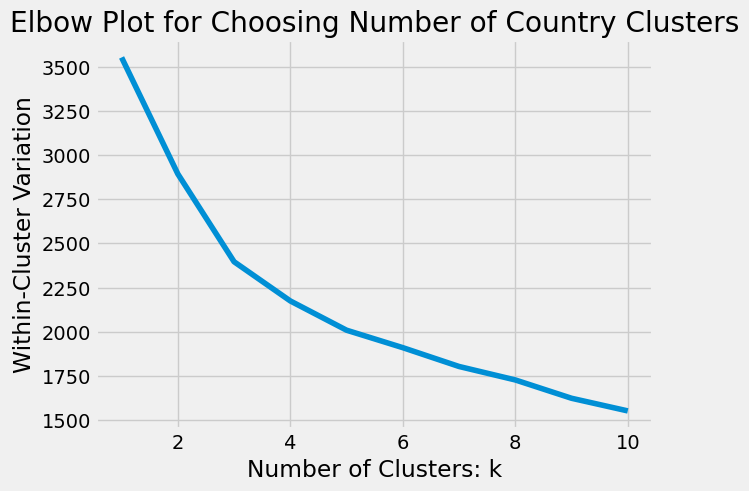
The elbow of this plot is not as clear as the plot from the previous section. It looks to be somewhere between 3 and 5. We will choose \(k = 4\) clusters for our data, since 4 is in the middle.
Training Our Model#
Now that we have chosen k, we can use KMeans to cluster our dataset into 4 clusters. The attribute .labels_ shows us the cluster membership for each row of countries proc.
kmeans = KMeans(n_clusters=4, n_init=10)
kmeans.fit(countries_proc)

kmeans.labels_
array([0, 2, 1, 0, 1, 1, 2, 2, 1, 1, 1, 2, 2, 2, 0, 1, 1, 2, 0, 0, 0, 1,
       0, 2, 2, 3, 1, 0, 2, 2, 2, 2, 0, 2, 1, 1, 2, 0, 1, 2, 2, 0, 0, 2,
       2, 0, 2, 1, 0, 1, 2, 2, 3, 1, 1, 1, 2, 2, 2, 2, 1, 1, 0, 1, 1, 0,
       2, 1, 2, 2, 0, 0, 1, 0, 2, 2, 1, 1, 1, 1, 0, 1, 1, 2, 1, 0, 0, 2,
       1, 1, 0, 1, 2, 1, 2, 2, 1, 2, 1, 0, 1, 0, 2, 0, 2, 2, 2, 1, 2, 2,
       1, 0, 2, 2, 2, 1, 1, 0, 1, 0, 0, 1, 1, 1, 0, 1, 1, 2, 3, 2, 1, 0],
      dtype=int32)
We can investigate which countries were clustered together using the country_names data which we extracted from our original dataset.
Cluster 0 seems to contain mostly European countries.
country_names[kmeans.labels_ == 0]
0                           Afghanistan
3                                Angola
14                                Benin
18                         Burkina Faso
19                              Burundi
20                          Ivory Coast
22                             Cameroon
27                Republic of the Congo
32     Democratic Republic of the Congo
37                             Ethiopia
41                                Gabon
42                           The Gambia
45                                Ghana
48                               Guinea
62                                Kenya
65                                 Laos
70                           Madagascar
71                               Malawi
73                                 Mali
80                           Mozambique
85                                Niger
86                              Nigeria
90                     Papua New Guinea
99                               Rwanda
101                             Senegal
103                        Sierra Leone
111                               Sudan
117                            Tanzania
119                          East Timor
120                                Togo
124                              Uganda
131                              Zambia
Name: Country, dtype: object
Cluster 1 contains many Middle Eastern and Eastern European countries as well as Southern and Central American countries.
country_names[kmeans.labels_ == 1]
2                   Algeria
4                 Argentina
5                   Armenia
8                Azerbaijan
9                   Bahrain
10               Bangladesh
15                 Botswana
16                   Brazil
21               Cape Verde
26                 Colombia
34       Dominican Republic
35                    Egypt
38                     Fiji
47                Guatemala
49                 Honduras
53                Indonesia
54                     Iran
55                     Iraq
60                   Jordan
61               Kazakhstan
63                   Kuwait
64               Kyrgyzstan
67                  Lebanon
72                 Malaysia
76                   Mexico
77                  Moldova
78                 Mongolia
79                  Morocco
81                  Myanmar
82                    Nepal
84                Nicaragua
88                     Oman
89                 Pakistan
91                 Paraguay
93              Philippines
96                    Qatar
98                   Russia
100            Saudi Arabia
107            South Africa
110               Sri Lanka
115                   Syria
116              Tajikistan
118                Thailand
121     Trinidad and Tobago
122                 Tunisia
123                  Turkey
125                 Ukraine
126    United Arab Emirates
130                 Vietnam
Name: Country, dtype: object
Cluster 2 contains mostly African countries.
country_names[kmeans.labels_ == 2]
1                  Albania
6                Australia
7                  Austria
11                Barbados
12                 Belgium
13                  Belize
17                Bulgaria
23                  Canada
24                   Chile
28              Costa Rica
29                 Croatia
30                  Cyprus
31          Czech Republic
33                 Denmark
36                 Estonia
39                 Finland
40                  France
43                 Georgia
44                 Germany
46                  Greece
50                 Hungary
51                 Iceland
56     Republic of Ireland
57                  Israel
58                   Italy
59                 Jamaica
66                  Latvia
68               Lithuania
69              Luxembourg
74                   Malta
75               Mauritius
83             New Zealand
87                  Norway
92                    Peru
94                  Poland
95                Portugal
97                 Romania
102                 Serbia
104              Singapore
105               Slovakia
106               Slovenia
108            South Korea
109                  Spain
112               Suriname
113                 Sweden
114            Switzerland
127         United Kingdom
129                Uruguay
Name: Country, dtype: object
China, India and the United States make up their own cluster.
country_names[kmeans.labels_ == 3]
25             China
52             India
128    United States
Name: Country, dtype: object
The map below shows which countries are assigned to each cluster. Interestingly, the clustering seems to have some geographic meaning. Countries close together on the map tend to belong to the same cluster.
Show code cell source
import plotly.express as px

dat = pd.DataFrame({'country_names': country_names, 'cluster': np.array([str(lab) for lab in kmeans.labels_])})

fig = px.choropleth(dat, locations="country_names",
                    locationmode='country names',
                    color="cluster",
                    color_discrete_sequence=["#D81B60","#1E88E5","#FFC107","#004D40"],
                    hover_name="country_names",
                    category_orders={"cluster":["0","1","2","3"]})
fig.update_layout(legend_title_text='Cluster Membership')

fig.show()
Disadvantages of K-Means Clustering#
As we discussed previously, k-means clustering has several disadvantages. It does not always converge to a solution that provides the global minimum within-cluster variation. Because of this, it can also give differing solutions depending on the initial starting points. In addition, the k-means algorithm requires the user to specify the number of clusters, which may not always be obvious, especially for data with high dimensionality. In the next section, we will discuss another clustering method that does not require you to specify a number of clusters: hierarchical clustering.