18.1. Correlation vs. Regression

Last chapter we saw that correlations can tell us about the strength of a linear relationship between variables. However, the correlation coefficient is far from everything when it comes to linear relationships. For instance, comparing the two data sets we see that even though the data sets are different the correlation coefficients are identical.

x1 = np.arange(10, 20)
y1 = np.array([19, 23, 22, 27, 30, 24, 28, 34, 40, 41])
r1 = np.corrcoef(x1,y1)[0,1]
print("r1 = ",r1)

x2 = np.arange(10, 20)
y2 = np.array([ 73,  89,  85, 105, 117,  93, 109, 133, 157, 161])
r2 = np.corrcoef(x2,y2)[0,1]
print("r2 = ",r2)

r1 =  0.9156112067119645
r2 =  0.9156112067119645

Looking at a graph of the above data sets we can see though that the relationship between \(x\) and \(y\) are different.

18.2. Finding Relationships

The difference between the two examples is that even though the correlation coefficient and hence the strength of the linear relationship between \(X\) and \(Y\) are the same, the relationship itself is different.

The difference between a linear relationship and a correlation coefficient is most easily seen in the case of perfectly correlated data.

x3 = np.arange(0, 10)
y3 = np.arange(1,21,2)
r3 = np.corrcoef(x3,y3)[0,1]

x4 = np.arange(0, 10)
y4 = np.arange(-2,38,4)
r4 = np.corrcoef(x4,y4)[0,1]

print("r3 = ", round(r3,4))
print("r4 = ", round(r4,4))

plt.plot(x3, y3, "o");
plt.plot(x4, y4, "o");

r3 =  1.0
r4 =  1.0

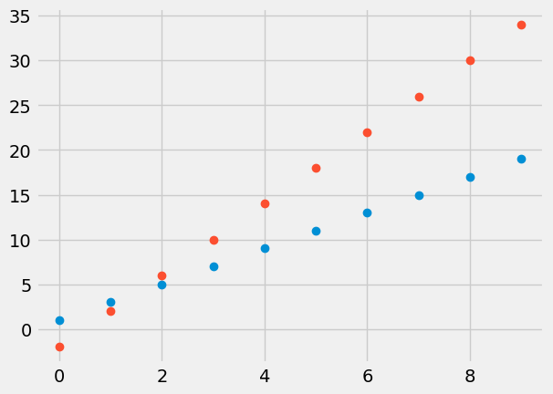
Here we see that though the correlation coefficients are both \(1\), the first data set lies on the line \(y = 2 x+1\) and for the second data set we have \(y = 4x-2\). The question remains how we can determine a relationship between \(x\) and \(y\) in general for non-perfectly correlated data.

For instance, look at the data below, along with the trend lines. Which trend line do you think best captures the relationship between the points?

While it might be hard to pinpoint the best one, some are clearly worse than others.